How Do Function Vectors Come into Being and Where Do They Live?
 Shantang Street, Suzhou.
This blog post documents an exploration undertaken from November 2025 to February 2026. The framework explored here has since been expanded to concept learning in an upcoming preprint. The author warmly thanks Alex Warstadt, Mikhail Belkin, Kyle Mahowald, Neil Mallinar, and Sasha Boguraev for their generous time and valuable feedback throughout this exploration.
1. Introduction
Function vectors (Todd et al., 2024) are compact, linear directions in activation space extracted from attention head outputs that causally induce specific task behaviors (such as antonym generation, country-capital retrieval, or translation) when added to the residual stream at inference time.
While the causal efficacy of function vectors in fully trained checkpoints is well established, fundamental questions remain regarding their developmental geometry during pre-training:
- How does the function vector evolve across pre-training? When does causal steering emerge, does discrete decision-flipping develop simultaneously with continuous logit push, and is there an abrupt transition during training?
- How does the model’s optimization geometry shape this development? How does the function vector relate to the principal directions of loss gradients as the model learns?
The initial intuition behind this investigation was straightforward: during pre-training, do task representations align with the loss landscape as gradients “carve out” functionality; and once the capability is consolidated, does the representation decouple from immediate loss gradients?
Our empirical results reveal a more nuanced picture. By tracing Function Vectors across 19 pre-training checkpoints (from Step 1 to Step 143,000, spanning five orders of magnitude on a logarithmic schedule) in Pythia-410M (evaluated on the antonym task) and Pythia-1B (evaluated across four core in-context learning tasks: antonym, country-capital, english-french, and present-past), and probing optimization geometry using the Average Gradient Outer Product (AGOP) (Radhakrishnan et al., 2024) alongside validation on a converged OLMo-1B model, we map the geometric lifecycle of task representations:
- In Pythia-410M, alignment with task gradient eigenspaces surges sharply around Step 1000 (within the first ~0.7% of training) before settling back to near-chance baseline at convergence.
- In Pythia-1B, alignment across four tasks exhibits a multi-peak dynamic: starting near chance, surging to an early peak at Step 1000–2000, experiencing a temporary dip during the middle training stage, and rebounding in late pre-training to settle consistently above chance baseline.
Key Takeaways
- Synchronized Transition within the First ~0.7% of Training: Function vector efficacy does not emerge gradually. Within the first ~0.7% of pre-training, the model undergoes an abrupt transition: the logit of the target token surges multiple-fold and cleanly diverges from isotropic random baselines, the optimal intervention site migrates from output layers to intermediate layers, and gradient alignment reaches an initial transient peak.
- Two-Stage Maturation (Logit Push vs. Decision Flipping): Continuous logit steering () separates from random control within the first ~0.7% of pre-training across all tasks. However, discrete argmax next-token classification flipping () matures significantly later and is model- and task-dependent. Crucially, elevating the target token’s logit score does not guarantee flipping the final classification: tasks like
present-pastandenglish-frenchachieve massive logit gains while exhibiting very weak top-1 separation from random control. - Subspace Energy Reorganization: During the early synchronized transition, the component residing in the task-irrelevant control subspace temporarily surges while the remaining orthogonal portion drops, before both settle back toward baseline. Throughout pre-training, the component parallel to task gradients accounts for only ~9–14% of total energy on Pythia-410M (), yet drives the majority of late-stage discrete classification flips, showing that alignment with gradient directions is far more consequential for accuracy than the total energy allocated to that component.
- Low-Rank Concentration: The function vector aligns predominantly with the leading few principal gradient directions, rapidly decaying to chance baseline across higher subspace dimensions.
- Metric-Specific Subspace Alignment: While the majority (73%–79%) of the vector’s energy resides in directions orthogonal to task gradients (driving continuous logit scale on Pythia-410M and OLMo-1B), the component parallel to task gradients is the primary driver of discrete classification flips. In late pre-training, isolating and normalizing the gradient-parallel component () outperforms the intact Function Vector in discrete argmax accuracy () at optimal intervention layers on Pythia-410M and converged OLMo-1B (on Pythia-1B, this advantage is task-dependent, holding on
country-capital,present-past, and late-stageantonym, but notenglish-french). On continuous logit steering (), however, the intact Function Vector remains superior on Pythia-410M and OLMo-1B across Steps 1000 to 143,000.
2. Setup & Framework
2.1 Models, Tasks, and Extraction
Primary Trajectory Models:
EleutherAI/pythia-410m(Biderman et al., 2023 layers, ), evaluated across 19 checkpoints onantonym: .EleutherAI/pythia-1b(Biderman et al., 2023 layers, ), evaluated across the identical 19 checkpoints across four tasks (antonym,country-capital,english-french,present-past).
- Cross-Model Validation:
allenai/OLMo-1B-0724-hf(Groeneveld et al., 2024 layers evaluated, ) at its final converged checkpoint (step1454000-tokens3048B). Task Protocols: 10-shot in-context learning (). Extraction set: 128 prompts; Evaluation set: 200 held-out prompt pairs; Random seed: 42. In each evaluation prompt, 10 demonstration pairs are formatted sequentially followed by an incomplete query prompt (e.g., in
antonym):Q: flawed A: perfect Q: orthodox A: unorthodox ... (8 more demonstration pairs) Q: unrelated A:The model’s greedy completion is evaluated against the target token (
related, noting the leading space).- Function Vector: Constructed following the causal indirect effect protocol (Todd et al., 2024), summing the outputs of top attention heads (default: top 5 heads) at the final token position.
2.2 Gradient Sensitivity and AGOP
To capture the model’s loss landscape geometry, we compute the Average Gradient Outer Product (AGOP) matrix with respect to the attention module output at the final token position under next-token cross-entropy loss as an empirical average over demonstration prompts:
Here, is the scalar cross-entropy loss on the target token. We use the leading orthonormal eigenvectors of (sorted by descending eigenvalue ) as the principal gradient subspace basis for projection and alignment measurements.
We construct two distinct AGOP matrices per layer:
- Task AGOP (): Computed over clean task ICL prompts, spanning the task-specific gradient subspace .
- Control-data AGOP (): Computed over length-matched uniform random token prompts with identical sequence lengths but arbitrary vocabulary tokens, defining a task-irrelevant baseline subspace .
Both AGOP and FV extraction use only the 128-prompt extraction set; the 200 evaluation prompt pairs remain strictly held-out.
2.3 Tri-Orthogonal Subspace Decomposition
To isolate where causal function resides relative to optimization gradients, we decompose the full Function Vector into three components via sequential projection. The construction strictly guarantees that is orthogonal to the remainder and that is orthogonal to :11 Sequential projection strictly guarantees that and . However, this construction does not generally guarantee that all three components are pairwise mutually orthogonal, because the Task and Control AGOP eigenspaces ( and ) can overlap. On Pythia-1B, the normalized subspace overlap ranges between and , which is small in absolute terms but above the random-subspace expectation of (). On Pythia-410M, we did not track subspace overlap across training.
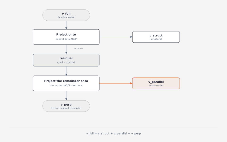
- Structural Component (): We first project the raw Function Vector onto the top- eigenspace of Control-data AGOP , yielding . This isolates the portion of the vector aligned with the length-matched random-token control baseline.
- Parallel Task Component (): We then take the structural remainder and project it directly onto the top- eigenspace of the original Task AGOP , yielding . Empirically, the task and control eigenspaces are nearly orthogonal in activation space, though this is an empirical property rather than an architectural constraint.
- Task-Orthogonal Remainder (): The remaining residual vector . By construction, is strictly orthogonal to the top Task AGOP subspace , and is approximately orthogonal to to the extent that task and control eigenspaces are empirically near-orthogonal in activation space.
To test causal behavior without magnitude confounds, each component is normalized to unit norm and scaled by , where is the layer-average activation norm evaluated at the final token position across evaluation prompts, before injection into the residual stream:
where is the steering intensity (default ).
3. Pre-Training Trajectory
Tracking the Function Vector across 19 pre-training checkpoints reveals that task capabilities do not accumulate linearly. Instead, the model undergoes a sharp, multi-metric transition at Step 1000 (the first ~0.7% of pre-training).
3.1 Causal Metrics and antonym Trajectory on Pythia-410M
When the extracted Function Vector is injected at layer with intensity , we evaluate two complementary causal metrics across 200 held-out evaluation pairs:
- (Continuous Steering Force): The change in the unnormalized logit score of the correct target token (). This measures whether the vector exerts directional push toward the target.
- (Discrete Decision Flipping): The change in greedy argmax accuracy. This measures whether the steering force is strong and calibrated enough to flip final token classification from incorrect to correct.
antonym, γ=1.0. Solid = median across the 24 layers (band = 25th–75th percentile); dashed = the single strongest layer. The two panels use different y-scales.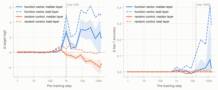
Data behind this figure
(target logit)
| step | FV median | FV best layer | random median | random best layer |
|---|---|---|---|---|
| 1 | -0.0344 | -0.0035 | 0.0147 | 0.0876 |
| 2 | -0.0331 | 0.0042 | 0.0148 | 0.0876 |
| 4 | -0.0338 | 0.0158 | 0.0163 | 0.0909 |
| 8 | -0.0146 | -0.0054 | 0.0209 | 0.0927 |
| 16 | -0.0456 | 0.0212 | 0.0060 | 0.0569 |
| 32 | -0.0676 | -0.0056 | 0.0108 | 0.0492 |
| 64 | -0.0323 | 0.0100 | 0.0125 | 0.0671 |
| 128 | 0.0143 | 0.0986 | 0.0416 | 0.1270 |
| 256 | 0.0381 | 0.4131 | 0.1577 | 0.5342 |
| 512 | 0.4727 | 0.6904 | 0.2881 | 0.9092 |
| 1000 | 2.7396 | 4.9398 | -0.3265 | 0.4320 |
| 2000 | 0.5405 | 2.0000 | -0.4448 | 1.2676 |
| 4000 | 0.7109 | 2.5273 | -0.7363 | 0.3809 |
| 8000 | 3.0322 | 5.6045 | -0.3806 | 0.3457 |
| 16000 | 2.9219 | 5.1465 | -1.2158 | -0.0410 |
| 32000 | 3.2871 | 6.1953 | -1.1279 | 0.0234 |
| 64000 | 1.8164 | 4.6406 | -1.5498 | -0.2246 |
| 120000 | 2.6641 | 5.1719 | -1.9824 | -0.0078 |
| 143000 | 1.9414 | 4.7617 | -1.5840 | -0.0312 |
(accuracy)
| step | FV median | FV best layer | random median | random best layer |
|---|---|---|---|---|
| 1 | 0.0000 | 0.0000 | 0.0000 | 0.0000 |
| 2 | 0.0000 | 0.0000 | 0.0000 | 0.0000 |
| 4 | 0.0000 | 0.0000 | 0.0000 | 0.0000 |
| 8 | 0.0000 | 0.0000 | 0.0000 | 0.0000 |
| 16 | 0.0000 | 0.0000 | 0.0000 | 0.0000 |
| 32 | 0.0000 | 0.0000 | 0.0000 | 0.0000 |
| 64 | 0.0000 | 0.0000 | 0.0000 | 0.0000 |
| 128 | 0.0000 | 0.0000 | 0.0000 | 0.0000 |
| 256 | 0.0000 | 0.0000 | 0.0000 | 0.0000 |
| 512 | 0.0000 | 0.0000 | 0.0000 | 0.0000 |
| 1000 | 0.0100 | 0.0300 | 0.0000 | 0.0100 |
| 2000 | 0.0000 | 0.0100 | 0.0000 | 0.0100 |
| 4000 | 0.0050 | 0.0400 | -0.0100 | 0.0100 |
| 8000 | -0.0100 | 0.0200 | -0.0100 | 0.0000 |
| 16000 | 0.0050 | 0.1100 | 0.0000 | 0.0100 |
| 32000 | 0.0150 | 0.2000 | 0.0000 | 0.0100 |
| 64000 | 0.0250 | 0.1700 | 0.0000 | 0.0100 |
| 120000 | 0.0750 | 0.4100 | 0.0000 | 0.0100 |
| 143000 | 0.0250 | 0.2900 | 0.0000 | 0.0100 |
Examining the trajectory in Pythia-410M on antonym reveals several key observations:
- The Step 1000 Transition: Read the onset against the random control, not against zero. Up to Step 512 the function vector does no more than an isotropic random vector of the same length (where the random control peak is vs for the function vector), so the minor lift before Step 1000 is not specific to the function vector. Across all 24 layers, the cross-layer median leaps from at Step 512 to at Step 1000. Concurrently, the optimal injection site shifts from the final output layer (Layer 23) to intermediate processing layers (Layer 10). Looking at the single strongest layer per checkpoint, the peak effect leaps by (from at Layer 23 at Step 512 to at Layer 10 at Step 1000). Note that is the peak at Step 1000; the global trajectory peak across all checkpoints reaches at Layer 9 at Step 32,000.
- Delayed Decision-Flipping Maturation: While directional logit force emerges at Step 1000, discrete next-token classification flipping develops much later. At Step 1000, at Layer 10 is only (2 out of 200 evaluation prompt pairs). From Steps 1000 to 8000, the gap over random control remains small and non-monotonic (0.020 to 0.030, returning to 0.000 at Step 2000). The first checkpoint where the gap reaches and remains sustained above that level is Step 16,000 ( peak at Layer 9 vs for random control), eventually reaching a peak of at Step 120,000.
3.2 Multi-Task Replication on Pythia-1B
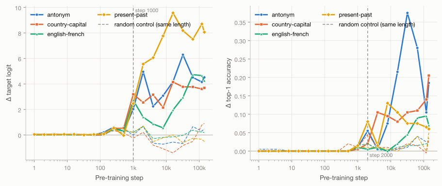
Does this early transition generalize beyond the antonym task? Evaluating Pythia-1B across 19 checkpoints on four distinct tasks demonstrates that this two-stage causal maturation is a general property of pre-training dynamics.
Data behind this figure
(target logit)
| step | antonym FV | antonym rand | country-capital FV | country-capital rand | english-french FV | english-french rand | present-past FV | present-past rand |
|---|---|---|---|---|---|---|---|---|
| 1 | 0.0136 | 0.0598 | 0.0441 | 0.0289 | 0.0135 | 0.0209 | 0.0403 | 0.0641 |
| 2 | 0.0503 | 0.0597 | 0.0296 | 0.0289 | 0.0136 | 0.0208 | 0.0270 | 0.0642 |
| 4 | 0.0548 | 0.0594 | 0.0652 | 0.0288 | 0.0138 | 0.0207 | 0.0301 | 0.0638 |
| 8 | 0.0380 | 0.0426 | 0.0354 | 0.0280 | 0.0212 | 0.0148 | 0.0496 | 0.0493 |
| 16 | 0.0223 | 0.0179 | 0.0340 | 0.0396 | 0.0172 | 0.0293 | 0.0506 | 0.0338 |
| 32 | 0.0157 | 0.0260 | 0.0230 | 0.0498 | 0.0039 | 0.0221 | -0.0002 | 0.0389 |
| 64 | -0.0018 | 0.0256 | -0.0138 | 0.0493 | 0.0237 | 0.0240 | 0.0392 | 0.0598 |
| 128 | 0.2100 | 0.1897 | 0.0007 | 0.1027 | 0.0563 | 0.0612 | 0.0735 | 0.1693 |
| 256 | 0.6162 | 0.5703 | 0.5097 | 0.3373 | 0.4878 | 0.3882 | 0.5420 | 0.5776 |
| 512 | 0.2803 | 0.4482 | 0.5352 | 0.1641 | 0.3047 | 0.3252 | -0.0347 | 0.4773 |
| 1000 | 2.0293 | 0.0059 | 3.1914 | -0.2461 | 2.7178 | 0.2188 | 2.4668 | 0.1660 |
| 2000 | 4.9541 | 0.6836 | 2.5469 | 0.2188 | 1.3999 | 0.6650 | 5.5596 | 0.7080 |
| 4000 | 2.2441 | -0.6445 | 3.1562 | -0.7930 | 0.8643 | -0.2910 | 6.0605 | -0.5176 |
| 8000 | 3.0781 | -0.7207 | 2.1484 | -1.0781 | 0.5557 | -0.1895 | 7.7617 | -0.2324 |
| 16000 | 4.1816 | -0.5547 | 4.1484 | -1.4062 | 1.9619 | -0.1445 | 9.5684 | 0.0098 |
| 32000 | 6.2930 | -0.6758 | 3.7773 | -0.8203 | 2.9512 | -0.0264 | 8.1855 | -0.6074 |
| 64000 | 4.5098 | 0.6543 | 3.7695 | -0.5039 | 4.7324 | 0.3750 | 7.5078 | -0.2617 |
| 120000 | 4.1543 | 0.3027 | 3.6094 | 0.7812 | 4.6582 | 0.2188 | 8.7031 | -0.3398 |
| 143000 | 4.5195 | 0.4766 | 3.6914 | 0.9023 | 4.2676 | 0.1973 | 8.0625 | -0.5078 |
(accuracy)
| step | antonym FV | antonym rand | country-capital FV | country-capital rand | english-french FV | english-french rand | present-past FV | present-past rand |
|---|---|---|---|---|---|---|---|---|
| 1 | 0.0000 | 0.0050 | 0.0000 | 0.0000 | 0.0000 | 0.0000 | 0.0000 | 0.0000 |
| 2 | 0.0000 | 0.0050 | 0.0000 | 0.0000 | 0.0000 | 0.0000 | 0.0000 | 0.0000 |
| 4 | 0.0000 | 0.0050 | 0.0000 | 0.0000 | 0.0000 | 0.0000 | 0.0000 | 0.0000 |
| 8 | 0.0000 | 0.0000 | 0.0000 | 0.0000 | 0.0000 | 0.0000 | 0.0000 | 0.0000 |
| 16 | 0.0000 | 0.0000 | 0.0000 | 0.0000 | 0.0000 | 0.0000 | 0.0000 | 0.0000 |
| 32 | 0.0000 | 0.0000 | 0.0000 | 0.0000 | 0.0000 | 0.0000 | 0.0000 | 0.0000 |
| 64 | 0.0000 | 0.0000 | 0.0000 | 0.0000 | 0.0000 | 0.0000 | 0.0000 | 0.0000 |
| 128 | 0.0000 | 0.0000 | 0.0000 | 0.0000 | 0.0000 | 0.0000 | 0.0000 | 0.0000 |
| 256 | 0.0000 | 0.0000 | 0.0000 | 0.0000 | 0.0000 | 0.0000 | 0.0000 | 0.0000 |
| 512 | 0.0000 | 0.0000 | 0.0000 | 0.0200 | 0.0000 | 0.0000 | 0.0000 | 0.0000 |
| 1000 | 0.0100 | 0.0050 | 0.0050 | 0.0100 | 0.0100 | 0.0150 | 0.0150 | 0.0100 |
| 2000 | 0.0550 | 0.0200 | 0.0200 | 0.0450 | 0.0050 | 0.0200 | 0.0800 | 0.0100 |
| 4000 | 0.0050 | 0.0050 | 0.1050 | 0.0100 | 0.0100 | 0.0050 | 0.0150 | 0.0100 |
| 8000 | 0.0750 | 0.0000 | 0.0950 | 0.0100 | 0.0000 | 0.0000 | 0.1300 | 0.0050 |
| 16000 | 0.2150 | 0.0050 | 0.0800 | 0.0050 | 0.0200 | 0.0100 | 0.1050 | 0.0000 |
| 32000 | 0.3750 | 0.0100 | 0.1050 | 0.0200 | 0.0450 | 0.0150 | 0.0750 | 0.0150 |
| 64000 | 0.2800 | 0.0400 | 0.1100 | 0.0150 | 0.0900 | 0.0150 | 0.0750 | 0.0400 |
| 120000 | 0.1050 | 0.0250 | 0.1400 | -0.0050 | 0.0950 | 0.0200 | 0.0650 | 0.0000 |
| 143000 | 0.1850 | 0.0250 | 0.2050 | 0.0350 | 0.0700 | 0.0200 | 0.0600 | 0.0500 |
- Onset Relative to Random Control (Step 1000): Up to Step 512, the function vector and random control coincide in every task. At Step 1000, the task-specific logit effect cleanly separates from the random control across all four tasks, with surging to 2.0–3.2 (7–15 the control level).
- Task-Dependent Top-1 Maturation: Discrete next-token decision-flipping () remains at zero through Step 512. Here, separation is defined as the first checkpoint where the function vector’s exceeds that of a same-length random vector. This separation emerges between Steps 2000 and 4000 in three tasks (
antonym,country-capital, andpresent-past), whereas inenglish-frencha sustained gap above a single test flip does not establish until Step 32,000. - Logit Push Does Not Imply Decision Flipping: While the Function Vector reliably elevates the target token’s logit score, this directional push does not necessarily alter the greedy argmax prediction. While
country-capital( at Step 143k) andantonym() achieve substantial greedy argmax accuracy gains,english-french() and especiallypresent-past() exhibit very weak top-1 separation from random control (whose final baseline is ), despitepresent-pastachieving the largest logit effect of all four tasks ().
4. Optimization Geometry
How does the Function Vector align with the model’s loss landscape during training? We project the extracted FV onto the top- eigenspaces of Task AGOP () and Control-data AGOP ().
4.1 Pythia-410M Alignment Trajectory
On Pythia-410M (), we track the alignment of the Function Vector with AGOP eigenspaces across training steps compared against both an empirical isotropic random-vector null control and the analytic chance baseline (representing the root-mean-square alignment for an isotropic random vector; see Appendix for proof sketch).
antonym, k=128. Line = median across the 24 layers; band = 25th–75th percentile. Solid = the function vector, dashed = an isotropic random vector of the same length. Blue and orange measure alignment with the task AGOP subspace, green and amber with the control AGOP subspace. The chance level is , the root-mean-square alignment a randomly drawn direction achieves with any 128-dimensional subspace of a 1024-dimensional space.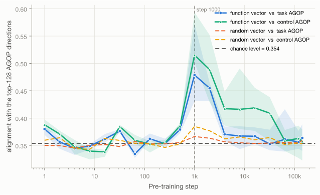
Data behind this figure
| step | FV vs task | random vs task | FV vs control | random vs control | FV - random | ratio FV/random | FV: control - task | random: control - task |
|---|---|---|---|---|---|---|---|---|
| 1 | 0.3800 | 0.3501 | 0.3878 | 0.3595 | 0.0299 | 1.0854 | 0.0078 | 0.0094 |
| 2 | 0.3565 | 0.3497 | 0.3709 | 0.3641 | 0.0068 | 1.0196 | 0.0144 | 0.0144 |
| 4 | 0.3447 | 0.3453 | 0.3478 | 0.3442 | -0.0006 | 0.9982 | 0.0031 | -0.0012 |
| 8 | 0.3491 | 0.3500 | 0.3397 | 0.3430 | -0.0009 | 0.9973 | -0.0094 | -0.0070 |
| 16 | 0.3618 | 0.3521 | 0.3383 | 0.3628 | 0.0097 | 1.0275 | -0.0235 | 0.0107 |
| 32 | 0.3762 | 0.3479 | 0.3849 | 0.3592 | 0.0283 | 1.0815 | 0.0087 | 0.0113 |
| 64 | 0.3345 | 0.3573 | 0.3594 | 0.3541 | -0.0228 | 0.9363 | 0.0249 | -0.0032 |
| 128 | 0.3622 | 0.3531 | 0.3525 | 0.3526 | 0.0091 | 1.0258 | -0.0096 | -0.0005 |
| 256 | 0.3532 | 0.3528 | 0.3545 | 0.3464 | 0.0003 | 1.0009 | 0.0013 | -0.0065 |
| 512 | 0.3791 | 0.3553 | 0.3861 | 0.3529 | 0.0238 | 1.0669 | 0.0070 | -0.0024 |
| 1000 | 0.4788 | 0.3663 | 0.5153 | 0.3848 | 0.1125 | 1.3070 | 0.0365 | 0.0185 |
| 2000 | 0.4547 | 0.3632 | 0.4887 | 0.3769 | 0.0915 | 1.2519 | 0.0340 | 0.0137 |
| 4000 | 0.3703 | 0.3567 | 0.4173 | 0.3620 | 0.0136 | 1.0381 | 0.0469 | 0.0053 |
| 8000 | 0.3673 | 0.3549 | 0.4161 | 0.3655 | 0.0124 | 1.0349 | 0.0488 | 0.0107 |
| 16000 | 0.3669 | 0.3537 | 0.4186 | 0.3603 | 0.0132 | 1.0374 | 0.0517 | 0.0066 |
| 32000 | 0.3526 | 0.3544 | 0.4090 | 0.3646 | -0.0017 | 0.9951 | 0.0564 | 0.0102 |
| 64000 | 0.3612 | 0.3557 | 0.3584 | 0.3516 | 0.0055 | 1.0155 | -0.0028 | -0.0041 |
| 120000 | 0.3561 | 0.3546 | 0.3629 | 0.3545 | 0.0015 | 1.0043 | 0.0068 | -0.0001 |
| 143000 | 0.3638 | 0.3591 | 0.3575 | 0.3530 | 0.0047 | 1.0131 | -0.0063 | -0.0061 |
The measured random control confirms the chance baseline empirically, sitting 2–4% above the analytic line. In the function vector trajectory:
- Alignment with Task AGOP rises above the random control strictly at Steps 1000 and 2000 (reaching and , corresponding to gaps of and over the measured random control).
- From Step 4000 onward, the gap narrows to (comparable to early baseline fluctuations), and by Step 143,000 it settles at (a gap of over the measured random control of ). Thus, by the end of training, the function vector is no more aligned with task loss gradients than a random direction.
- Notably, during the middle training stage (Steps 1000–32,000), the Function Vector aligns more strongly with the Control-data AGOP than with the Task AGOP (e.g., at Step 1000: vs , a gap of ; at Step 32,000: vs , a gap of ). The isotropic random vector shows only a small preference for the control subspace ( to ), demonstrating that this preference is not purely an artifact of the control subspace itself. The precise mechanism behind this elevated control alignment remains an open question. At convergence, alignment with both subspaces returns to chance level ( for Control-data AGOP and for Task AGOP).
4.2 Multi-Task Alignment on Pythia-1B
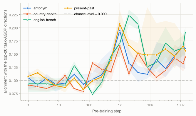
On Pythia-1B (), we evaluate AGOP alignment across all four tasks against the analytic chance baseline .
Data behind this figure
| step | antonym | antonym xchance | country-capital | country-capital xchance | english-french | english-french xchance | present-past | present-past xchance |
|---|---|---|---|---|---|---|---|---|
| 1 | 0.1045 | 1.0575 | 0.0909 | 0.9198 | 0.0932 | 0.9432 | 0.1073 | 1.0853 |
| 2 | 0.0912 | 0.9232 | 0.0878 | 0.8883 | 0.0931 | 0.9424 | 0.1143 | 1.1570 |
| 4 | 0.1038 | 1.0508 | 0.0842 | 0.8518 | 0.0932 | 0.9428 | 0.1014 | 1.0257 |
| 8 | 0.0920 | 0.9312 | 0.0914 | 0.9249 | 0.0913 | 0.9239 | 0.0895 | 0.9061 |
| 16 | 0.0945 | 0.9565 | 0.1084 | 1.0966 | 0.0908 | 0.9192 | 0.0862 | 0.8726 |
| 32 | 0.1112 | 1.1249 | 0.0841 | 0.8508 | 0.1283 | 1.2981 | 0.1040 | 1.0519 |
| 64 | 0.0925 | 0.9362 | 0.0783 | 0.7928 | 0.1031 | 1.0435 | 0.0824 | 0.8342 |
| 128 | 0.1015 | 1.0269 | 0.1327 | 1.3426 | 0.0734 | 0.7432 | 0.0989 | 1.0007 |
| 256 | 0.1104 | 1.1176 | 0.1209 | 1.2230 | 0.0958 | 0.9694 | 0.1061 | 1.0737 |
| 512 | 0.1390 | 1.4066 | 0.1161 | 1.1751 | 0.1459 | 1.4763 | 0.1376 | 1.3923 |
| 1000 | 0.1944 | 1.9673 | 0.1651 | 1.6708 | 0.1700 | 1.7206 | 0.2071 | 2.0959 |
| 2000 | 0.1328 | 1.3436 | 0.1126 | 1.1393 | 0.2240 | 2.2668 | 0.1666 | 1.6859 |
| 4000 | 0.1145 | 1.1589 | 0.1522 | 1.5400 | 0.2062 | 2.0869 | 0.1509 | 1.5271 |
| 8000 | 0.1112 | 1.1255 | 0.1240 | 1.2552 | 0.1254 | 1.2692 | 0.1481 | 1.4984 |
| 16000 | 0.1391 | 1.4075 | 0.1055 | 1.0674 | 0.1335 | 1.3512 | 0.1482 | 1.4994 |
| 32000 | 0.1221 | 1.2358 | 0.1188 | 1.2018 | 0.1708 | 1.7282 | 0.1592 | 1.6113 |
| 64000 | 0.1468 | 1.4852 | 0.1423 | 1.4397 | 0.1557 | 1.5759 | 0.1458 | 1.4755 |
| 120000 | 0.1641 | 1.6603 | 0.1317 | 1.3328 | 0.1616 | 1.6355 | 0.1640 | 1.6600 |
| 143000 | 0.1606 | 1.6249 | 0.1440 | 1.4573 | 0.1917 | 1.9398 | 0.1561 | 1.5792 |
All four tasks scatter around chance until Step 512; early excursions (such as country-capital at Step 128 reaching chance) are transient and not sustained. From Step 512, all four tasks rise to a peak at Steps 1000–2000 at – chance (english-french peaking at Step 2000 at chance; antonym, country-capital, and present-past peaking at Step 1000 at – chance). The trajectories then experience dips that vary by task (troughing at Step 8000 for antonym and english-french, Step 16,000 for country-capital, and a shallow dip at Step 64,000 for present-past), before recovering in late training to settle consistently above chance baseline at convergence (– chance, ranging from to ).
The two models used different subspace truncation sizes ( for Pythia-410M, for Pythia-1B), so only the qualitative shapes and each model’s own endpoint relative to its baseline are comparable, not the raw peak heights. Unlike the 410M evaluations, these 1B runs did not record an empirical random-vector control, so the baseline shown is the analytic chance line.
4.3 Divergent Alignment Dynamics
Across the two model scales, the alignment between Function Vectors and task gradient eigenspaces shows distinct developmental trajectories:
- Pythia-410M exhibits a single-peak dynamic: alignment makes a single narrow departure from baseline strictly at Steps 1000–2000 before returning to near-chance levels for the remainder of training.
- Pythia-1B exhibits a multi-peak dynamic: alignment rises to an early peak at Steps 1000–2000, dips during intermediate steps, and rebounds in late pre-training to settle stably above chance.
5. Subspace Energy
To understand how the Function Vector distributes across the decomposed subspaces, we examine energy allocation across pre-training. For each component , its energy fraction is defined as its normalized squared norm, , such that the three components strictly sum to . For a single projection, this equals the squared cosine alignment with the subspace. Fixing on Pythia-410M (), the chance expected energy fraction for an isotropic random vector projected onto the -dimensional control subspace is exactly . For the task-parallel component , the expected energy fraction is , where measures subspace overlap. For the task-orthogonal remainder (), the expected energy fraction is , achieving the lower bound of when the two subspaces are strictly orthogonal ().
antonym task). Shaded bands represent the interquartile range across network layers within a single checkpoint. Dashed reference lines denote random-vector baselines: represents the exact expectation for and an upper reference for , while marks the theoretical lower bound for .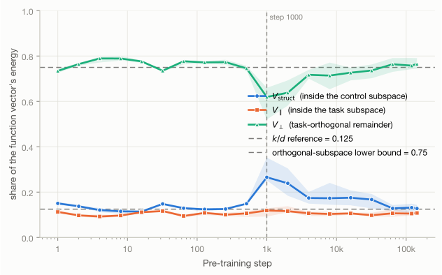
Data behind this figure
| step | V_struct | V_parallel | V_perp |
|---|---|---|---|
| 1 | 0.1504 | 0.1125 | 0.7345 |
| 2 | 0.1376 | 0.0975 | 0.7644 |
| 4 | 0.1210 | 0.0926 | 0.7893 |
| 8 | 0.1154 | 0.0971 | 0.7890 |
| 16 | 0.1145 | 0.1114 | 0.7763 |
| 32 | 0.1481 | 0.1166 | 0.7353 |
| 64 | 0.1291 | 0.0947 | 0.7769 |
| 128 | 0.1243 | 0.1086 | 0.7718 |
| 256 | 0.1256 | 0.1004 | 0.7731 |
| 512 | 0.1491 | 0.1064 | 0.7457 |
| 1000 | 0.2656 | 0.1190 | 0.6195 |
| 2000 | 0.2389 | 0.1161 | 0.6385 |
| 4000 | 0.1741 | 0.1067 | 0.7173 |
| 8000 | 0.1731 | 0.1037 | 0.7139 |
| 16000 | 0.1754 | 0.1062 | 0.7266 |
| 32000 | 0.1673 | 0.0982 | 0.7361 |
| 64000 | 0.1285 | 0.1067 | 0.7639 |
| 120000 | 0.1317 | 0.1054 | 0.7579 |
| 143000 | 0.1278 | 0.1081 | 0.7651 |
- Expected Energy Allocation in : Away from Step 1000, all three components sit near their expected random baselines. Across early and final checkpoints, the task-orthogonal remainder accounts for 73%–79% of total energy (at Step 143k, the cross-layer median reaches 76.5%, with Layer 10 at 73.3%). This sits near the random-vector expectation of .
- The Step 1000 Structural Reorganization: The primary departure occurs at Step 1000: the network-wide cross-layer median energy of rises to 26.6% (about chance expectation) while drops to 62.0%. At Layer 10, reaches 47.4% while falls to 39.4%. Throughout pre-training, the task-parallel component maintains a steady energy share of ~9–12% (cross-layer median 11.9% at Step 1000, 10.8% at Step 143k).
6. Low-Rank Concentration
How deeply does the Function Vector align with the Task AGOP eigenspace? By sweeping the truncation rank on Pythia-410M () at the final checkpoint (Step 143,000), we measure the Enrichment Ratio, defined as the energy fraction of in the top- Task AGOP subspace divided by the random chance baseline :
antonym, final checkpoint (step 143000). Band = 25th–75th percentile across layers.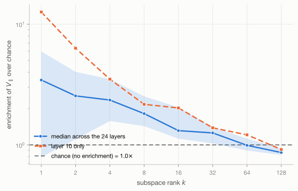
Data behind this figure
| k | median | p25 | p75 | layer 10 |
|---|---|---|---|---|
| 1 | 3.4485 | 0.7905 | 5.9439 | 12.6146 |
| 2 | 2.5487 | 1.1145 | 4.0335 | 6.3251 |
| 4 | 2.3543 | 1.5771 | 3.5085 | 3.5061 |
| 8 | 1.8170 | 1.4309 | 2.5285 | 2.1695 |
| 16 | 1.3142 | 1.1266 | 2.0446 | 2.0254 |
| 32 | 1.2575 | 1.0281 | 1.4109 | 1.3866 |
| 64 | 0.9925 | 0.8992 | 1.1279 | 1.2126 |
| 128 | 0.8651 | 0.8260 | 0.9370 | 0.9170 |
The Function Vector is concentrated along the leading 1 to 4 eigenvectors of the Task AGOP matrix:
- At , the cross-layer median reaches chance, while Layer 10 reaches (and deeper layers such as Layer 12 reach , Layer 13 reaches , and Layer 11 reaches ). Layer 10 is highlighted as the primary causal intervention site, not the maximum enrichment layer.
- By , the enrichment ratio falls below ( median, at Layer 10). This shows that the task-specific alignment is concentrated in the top few gradient directions, while higher-dimensional subspaces capture energy at or below chance expectation.
7. Component Causal Efficacy
When we isolate , , and , scale each to unit layer norm, and inject them individually at inference, how do their causal effects compare to the intact Function Vector?
antonym, k=128, γ=1.0. Solid with markers = the strongest layer at that checkpoint; faint dotted in the same colour = the median layer for the same component.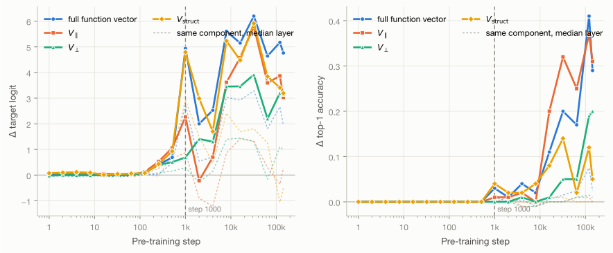
Data behind this figure
(target logit)
| step | full FV | V_parallel | V_perp | V_struct |
|---|---|---|---|---|
| 1 | -0.0035 | 0.0779 | -0.0224 | 0.0756 |
| 2 | 0.0042 | 0.0511 | 0.0035 | 0.0991 |
| 4 | 0.0158 | 0.0632 | -0.0070 | 0.1173 |
| 8 | -0.0054 | 0.0506 | -0.0078 | 0.0969 |
| 16 | 0.0212 | 0.0589 | 0.0004 | 0.0160 |
| 32 | -0.0056 | 0.0432 | -0.0069 | 0.0415 |
| 64 | 0.0100 | -0.0023 | 0.0177 | 0.0628 |
| 128 | 0.0986 | 0.1298 | 0.0994 | 0.0784 |
| 256 | 0.4131 | 0.5264 | 0.3965 | 0.4316 |
| 512 | 0.6904 | 1.0596 | 0.5098 | 0.9297 |
| 1000 | 4.9398 | 2.2699 | 0.6884 | 4.7914 |
| 2000 | 2.0000 | -0.2188 | 1.4082 | 2.9883 |
| 4000 | 2.5273 | 0.7031 | 1.3047 | 1.6992 |
| 8000 | 5.6045 | 3.6162 | 3.4521 | 5.2295 |
| 16000 | 5.1465 | 4.5801 | 3.4590 | 4.4785 |
| 32000 | 6.1953 | 5.7891 | 3.9141 | 5.9141 |
| 64000 | 4.6406 | 3.5938 | 2.1953 | 3.8438 |
| 120000 | 5.1719 | 3.8672 | 3.2031 | 3.4062 |
| 143000 | 4.7617 | 3.0273 | 3.1523 | 3.1914 |
(accuracy)
| step | full FV | V_parallel | V_perp | V_struct |
|---|---|---|---|---|
| 1 | 0.0000 | 0.0000 | 0.0000 | 0.0000 |
| 2 | 0.0000 | 0.0000 | 0.0000 | 0.0000 |
| 4 | 0.0000 | 0.0000 | 0.0000 | 0.0000 |
| 8 | 0.0000 | 0.0000 | 0.0000 | 0.0000 |
| 16 | 0.0000 | 0.0000 | 0.0000 | 0.0000 |
| 32 | 0.0000 | 0.0000 | 0.0000 | 0.0000 |
| 64 | 0.0000 | 0.0000 | 0.0000 | 0.0000 |
| 128 | 0.0000 | 0.0000 | 0.0000 | 0.0000 |
| 256 | 0.0000 | 0.0000 | 0.0000 | 0.0000 |
| 512 | 0.0000 | 0.0000 | 0.0000 | 0.0000 |
| 1000 | 0.0300 | 0.0100 | 0.0000 | 0.0400 |
| 2000 | 0.0100 | 0.0100 | 0.0000 | 0.0200 |
| 4000 | 0.0400 | 0.0200 | 0.0100 | 0.0200 |
| 8000 | 0.0200 | 0.0000 | 0.0000 | 0.0400 |
| 16000 | 0.1100 | 0.2000 | 0.0100 | 0.0800 |
| 32000 | 0.2000 | 0.3200 | 0.0500 | 0.1400 |
| 64000 | 0.1700 | 0.2500 | 0.0500 | 0.0200 |
| 120000 | 0.4100 | 0.3700 | 0.1900 | 0.1200 |
| 143000 | 0.2900 | 0.3100 | 0.2000 | 0.0500 |
Every component is injected at the same length (rescaled to times the layer’s mean activation norm), testing directional efficacy rather than magnitude:
- For continuous logit steering (), the cross-layer median reaches roughly half the single best layer (e.g., full FV at Step 32,000 has median vs peak ), indicating broadly distributed directional lift across layers.
- For discrete argmax classification (), the cross-layer median is essentially zero across all components, while the single strongest layer reaches (for the intact Function Vector at Layer 9 at Step 120,000) and (for isolated at Layer 9 at Step 32,000, where the cross-layer median is ). This shows that decision-flipping is concentrated in specific intermediate intervention layers.
7.1 Metric Divergence on Pythia-410M and OLMo-1B
Decomposing the Function Vector reveals a divergence between continuous logit steering and discrete classification success:
- Discrete Classification Success (): At the single best-performing intervention layer, isolated outperforms the intact Function Vector in 4 out of the final 5 pre-training checkpoints on Pythia-410M. At Step 32,000, peak (Layer 9) achieves , exceeding peak full FV ( at Layer 9). At convergence (Step 143k), remains superior ( at Layer 12 vs at Layer 9 for full FV). On converged OLMo-1B (
step1454000-tokens3048B), peak (Layer 6) achieves compared to for peak full FV at Layer 5 (a improvement). - Continuous Steering Force (): On Pythia-410M, across all 9 checkpoints from Step 1000 to 143,000 (following initial causal emergence), isolated never exceeds the intact Function Vector in continuous logit steering (0 out of 9 checkpoints). The full Function Vector consistently produces the largest raw logit shift on Pythia-410M and OLMo-1B because the orthogonal component also contributes continuous logit magnitude.
- Component Roles in Early vs. Late Training: At Step 1000 on Pythia-410M, accounts for the majority of the initial classification effect ( vs for and for , representing 80% of total top-1 flips). However, in late pre-training (Step 143k), accounts for the largest share of classification success (about 55% of the summed component effect, vs for and for ).
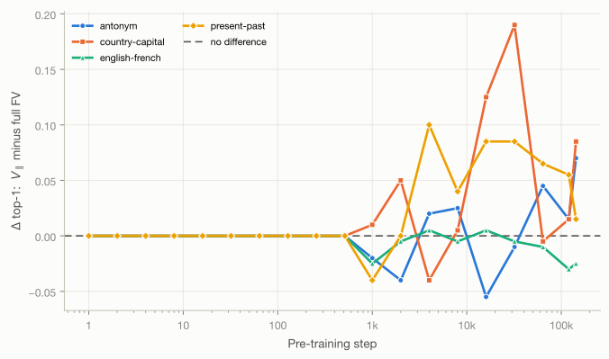
7.2 Cross-Task Component Advantage on Pythia-1B
To test whether isolating improves discrete accuracy across multiple tasks, we evaluate the difference in between the isolated task-parallel component and the intact Function Vector across 19 checkpoints in Pythia-1B ().
Data behind this figure
| step | antonym V_par | antonym full FV | antonym difference | country-capital V_par | country-capital full FV | country-capital difference | english-french V_par | english-french full FV | english-french difference | present-past V_par | present-past full FV | present-past difference |
|---|---|---|---|---|---|---|---|---|---|---|---|---|
| 1 | 0.0000 | 0.0000 | 0.0000 | 0.0000 | 0.0000 | 0.0000 | 0.0000 | 0.0000 | 0.0000 | 0.0000 | 0.0000 | 0.0000 |
| 2 | 0.0000 | 0.0000 | 0.0000 | 0.0000 | 0.0000 | 0.0000 | 0.0000 | 0.0000 | 0.0000 | 0.0000 | 0.0000 | 0.0000 |
| 4 | 0.0000 | 0.0000 | 0.0000 | 0.0000 | 0.0000 | 0.0000 | 0.0000 | 0.0000 | 0.0000 | 0.0000 | 0.0000 | 0.0000 |
| 8 | 0.0000 | 0.0000 | 0.0000 | 0.0000 | 0.0000 | 0.0000 | 0.0000 | 0.0000 | 0.0000 | 0.0000 | 0.0000 | 0.0000 |
| 16 | 0.0000 | 0.0000 | 0.0000 | 0.0000 | 0.0000 | 0.0000 | 0.0000 | 0.0000 | 0.0000 | 0.0000 | 0.0000 | 0.0000 |
| 32 | 0.0000 | 0.0000 | 0.0000 | 0.0000 | 0.0000 | 0.0000 | 0.0000 | 0.0000 | 0.0000 | 0.0000 | 0.0000 | 0.0000 |
| 64 | 0.0000 | 0.0000 | 0.0000 | 0.0000 | 0.0000 | 0.0000 | 0.0000 | 0.0000 | 0.0000 | 0.0000 | 0.0000 | 0.0000 |
| 128 | 0.0000 | 0.0000 | 0.0000 | 0.0000 | 0.0000 | 0.0000 | 0.0000 | 0.0000 | 0.0000 | 0.0000 | 0.0000 | 0.0000 |
| 256 | 0.0000 | 0.0000 | 0.0000 | 0.0000 | 0.0000 | 0.0000 | 0.0000 | 0.0000 | 0.0000 | 0.0000 | 0.0000 | 0.0000 |
| 512 | 0.0000 | 0.0000 | 0.0000 | 0.0000 | 0.0000 | 0.0000 | 0.0000 | 0.0000 | 0.0000 | 0.0000 | 0.0000 | 0.0000 |
| 1000 | -0.0100 | 0.0100 | -0.0200 | 0.0150 | 0.0050 | 0.0100 | -0.0150 | 0.0100 | -0.0250 | -0.0250 | 0.0150 | -0.0400 |
| 2000 | 0.0150 | 0.0550 | -0.0400 | 0.0700 | 0.0200 | 0.0500 | 0.0000 | 0.0050 | -0.0050 | 0.0800 | 0.0800 | 0.0000 |
| 4000 | 0.0250 | 0.0050 | 0.0200 | 0.0650 | 0.1050 | -0.0400 | 0.0150 | 0.0100 | 0.0050 | 0.1150 | 0.0150 | 0.1000 |
| 8000 | 0.1000 | 0.0750 | 0.0250 | 0.1000 | 0.0950 | 0.0050 | -0.0050 | 0.0000 | -0.0050 | 0.1700 | 0.1300 | 0.0400 |
| 16000 | 0.1600 | 0.2150 | -0.0550 | 0.2050 | 0.0800 | 0.1250 | 0.0250 | 0.0200 | 0.0050 | 0.1900 | 0.1050 | 0.0850 |
| 32000 | 0.3650 | 0.3750 | -0.0100 | 0.2950 | 0.1050 | 0.1900 | 0.0400 | 0.0450 | -0.0050 | 0.1600 | 0.0750 | 0.0850 |
| 64000 | 0.3250 | 0.2800 | 0.0450 | 0.1050 | 0.1100 | -0.0050 | 0.0800 | 0.0900 | -0.0100 | 0.1400 | 0.0750 | 0.0650 |
| 120000 | 0.1200 | 0.1050 | 0.0150 | 0.1550 | 0.1400 | 0.0150 | 0.0650 | 0.0950 | -0.0300 | 0.1200 | 0.0650 | 0.0550 |
| 143000 | 0.2550 | 0.1850 | 0.0700 | 0.2900 | 0.2050 | 0.0850 | 0.0450 | 0.0700 | -0.0250 | 0.0750 | 0.0600 | 0.0150 |
The component advantage in Pythia-1B shows substantial task-dependent heterogeneity:
- In
country-capitalandpresent-past, the isolated component establishes a stable late advantage (at Step 143,000, difference is and ). - In
antonym, the isolated component is below zero at Steps 16,000 () and 32,000 (), before turning positive from Step 64,000 onward (reaching at Step 143,000). - In
english-french, the isolated component never establishes an advantage over the intact vector, ending at at Step 143,000.
Furthermore, on continuous logit steering (), Pythia-1B exhibits dynamics distinct from Pythia-410M: on Pythia-1B, frequently exceeds the intact Function Vector in raw logit lift (e.g., at Step 64,000 across all four tasks). The claim that the intact Function Vector consistently produces larger logit shifts is specific to Pythia-410M and OLMo-1B (both evaluated on antonym).
7.3 Margin Selectivity and Classification Mechanics
Why does flip more discrete decisions despite producing a smaller raw target logit increase on Pythia-410M? An inspection of prediction margins () reveals how the three components navigate the trade-off between push magnitude and selectivity:
- At Step 32,000 (Layer 9), achieves the highest margin gain (, ) by combining strong target push () with moderate competitor lift (). In contrast, produces matching target push () but elevates competing logits heavily (, , ). Meanwhile, is the most selective (elevating competitors by only , ) but achieves a smaller raw margin () and flips very few decisions (, 2 of 200).
- At Step 143,000 (Layer 10), produces the largest margin gain (, shifting competing logits by , ), while and elevate competing logits by (, ) and (, ), respectively.
This pattern is corroborated in probability space by target-versus-rest log-odds (): at Step 32,000 (Layer 9), achieves compared to for and for .
These measurements show that discrete classification flipping requires both sufficient target push and selectivity against competitor elevation: pushes strongly but non-selectively, is selective but weak in raw margin at Step 32,000, and only satisfies both criteria at both checkpoints examined (note: tracks the maximum logit among non-target tokens, and the identity of this maximizing token may change before and after intervention).
8. Limitations
We explicitly state the empirical boundaries of this study:
- Model and Checkpoint Scope: Full developmental trajectories across 19 pre-training checkpoints are analyzed on Pythia-410M and Pythia-1B. Validation on OLMo-1B is restricted to its single converged checkpoint (
step1454000-tokens3048B), as intermediate pre-training checkpoints were not available. On Pythia-410M, the control-aligned component plays a non-trivial causal role in the middle training stage that it does not retain at convergence; because OLMo-1B provides only a converged checkpoint, this mid-training trajectory has not yet been tested there. - Layer Variance vs. Statistical Error: Shaded bands in our figures represent the interquartile range (25th–75th percentile) across network layers within a single checkpoint run, illustrating how intervention efficacy varies across injection layers. They do not represent sampling variance across evaluation prompts or cross-seed training variance. The study plots no statistical error bars.
- Subspace Hyperparameters: The multi-task component advantage evaluation on Pythia-1B was conducted with a single random seed and fixed subspace rank .
9. Conclusion
By observing Function Vector causal efficacy throughout pre-training and decomposing vectors against empirical loss gradient eigenspaces (AGOP), we map the developmental geometry of linear task representations:
- Phase Transition at Step 1000 (~0.7% of Pre-Training): In both Pythia-410M and Pythia-1B, task-directed continuous steering () cleanly separates from isotropic random baselines, coinciding with a shift in optimal injection sites to intermediate layers and an initial peak in gradient subspace alignment.
- Staggered Emergence of Logit Steering vs. Decision Flipping: Discrete classification flipping () develops substantially later (Steps 2000–4000 in Pythia-1B, Step 16,000 in Pythia-410M). Strong logit push does not guarantee argmax decision flips, as shown by weak top-1 separation on
english-frenchandpresent-past. - Divergent Alignment Dynamics: Pythia-410M exhibits a single-peak dynamic (a narrow departure strictly at Steps 1000–2000 before returning to chance baseline), while Pythia-1B displays a multi-peak trajectory that rebounds in late pre-training to settle stably above chance.
- Low-Rank Concentration: Gradient alignment is concentrated along the leading eigenvectors of the Task AGOP matrix (reaching enrichment at in Layer 10 of Pythia-410M), decaying to chance expectation across higher dimensions.
- Metric-Specific Subspace Specialization: Separating the task-parallel component () from the control subspace () and task-orthogonal nullspace () yields vectors that outperform intact Function Vectors in discrete classification success () at optimal intervention layers in late pre-training across Pythia-410M, converged OLMo-1B, and select Pythia-1B tasks, while intact Function Vectors maintain higher continuous logit push on Pythia-410M and OLMo-1B.
Appendix: Expected Energy Fraction Proof Sketches
The theoretical baselines for subspace energy and alignment derive from projection properties of isotropic random vectors:
Energy Fraction in a -Dimensional Subspace (): For a standard Gaussian random vector , the total energy . Projecting onto an arbitrary -dimensional subspace yields projected energy , while the orthogonal component . Since and are independent, the energy fraction follows a Beta distribution . Its expected value is:
The root-mean-square cosine alignment is .
Task-Parallel Component ():
where is the subspace overlap. Thus serves as an upper bound, with equality achieved if and only if the subspaces are strictly orthogonal ().
Task-Orthogonal Remainder ():
Thus serves as an exact lower bound, achieved if and only if the task and control subspaces are strictly orthogonal ().
References
- Todd, E., Li, M., Sen Sharma, A., Mueller, A., Wallace, B. C., & Bau, D. (2024). Function Vectors in Large Language Models. The Twelfth International Conference on Learning Representations (ICLR 2024). https://openreview.net/forum?id=AwyxtyMwaG
- Radhakrishnan, A., Beaglehole, D., Pandit, P., & Belkin, M. (2024). Mechanism for feature learning in neural networks and backpropagation-free machine learning models. Science, 383(6690), 1461–1467. https://doi.org/10.1126/science.adi5639
- Biderman, S., Schoelkopf, H., Anthony, Q. G., Bradley, H., O’Brien, K., Hallahan, E., Khan, M. A., Purohit, S., Prashanth, U. S., Raff, E., Skowron, A., Sutawika, L., & Van Der Wal, O. (2023). Pythia: A Suite for Analyzing Large Language Models Across Training and Scaling. Proceedings of the 40th International Conference on Machine Learning, PMLR 202, 2397–2430. https://proceedings.mlr.press/v202/biderman23a.html
- Groeneveld, D., Beltagy, I., Walsh, E., Bhagia, A., Kinney, R., Tafjord, O., Jha, A., Ivison, H., Magnusson, I., Wang, Y., Arora, S., Atkinson, D., Authur, R., Chandu, K., Cohan, A., Dumas, J., Elazar, Y., Gu, Y., Hessel, J., … Hajishirzi, H. (2024). OLMo: Accelerating the Science of Language Models. Proceedings of the 62nd Annual Meeting of the Association for Computational Linguistics (Volume 1: Long Papers), 15789–15809. https://doi.org/10.18653/v1/2024.acl-long.841
Cite this post
@misc{wang2026functionvectors,
  author       = {Yupei Wang},
  title        = {How Do Function Vectors Come into Being and Where Do They Live?},
  year         = {2026},
  month        = {aug},
  doi          = {10.5281/zenodo.22109632},
  howpublished = {\url{https://ypwang.one/Blog/fv-agop-dev-interp/}},
  urldate      = {2026-08-25},
  note         = {Blog post},
}